EXPERT KNOWLEDGE AT A GLANCE

Category: Machine learning (Page 1 of 3)

NumPy vs Pandas – Which is used When?

NumPy vs Pandas – Since in our time in every science and economic branch ever larger amounts of data accumulate, which must be analyzed and managed performantly, the learning of a programming language has become interdisciplinary indispensable.

For many, Python is the first programming language in the classical sense, due to its beginner friendliness and mathematical focus. Python offers the possibility of accessing ready-made, optimized computational tools through the modular implementation of powerful mathematical libraries.
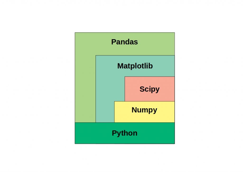
NumPy vs Pandas - The schme shows popular python libraries and their place in the Python ecosystem
NumPy vs Pandas – Their place in the Python ecosystem

However, this offer can also quickly become overwhelming. Which library, which framework is suitable for my purposes? Will I save myself work with this tool, or will I reach its limits? Here you can learn more about SciPy and why you should definitely prefer it over MATLAB and here we compared the two Python visualization methods matplotlib and seaborn. These Python libraries are absolutely compatible with each other and together they make a very interesting data science tool. NumPy and Pandas are perhaps two of the best-known python libraries. But what are the differences between them? We will get to the bottom of this question in this article.

What actually is NumPy?

NumPy stands for “Numerical Python” and is an open source Python library for array-based calculations. It was first released in 1995 as Numeric, making it the first implementation of a Python matrix package, and rereleased as NumPy in 2006. This library is intended to allow easy handling of vectors, matrices, or large multidimensional arrays in general.
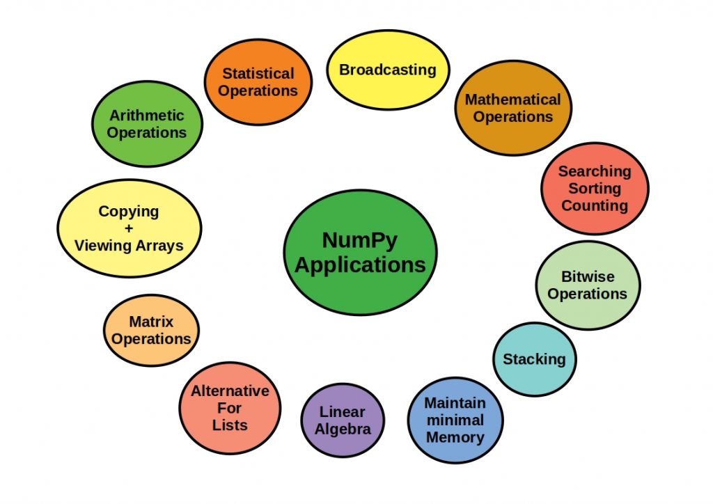
 

The scheme shows NumPys major applications
NumPy vs Pandas – Numpys Major Applications

For performance purposes, it is written in C, a deep, machine-oriented programming language. NumPy is compatible with a wide variety of Python libraries, some of which are also based on NumPy, adding further useful functions to its power, such as: Minimization, Regression, Fourier Transform

Python and Science

As mentioned earlier, Python is the programming language most intensively used in the application domain of scientific research across all disciplines for data processing and analysis. What is very interesting here is that the solution approaches are similar across disciplines at the data level. Thus, an exchange of ideas has become indispensable and leads more and more to a fusion of the sciences.

This is only mentioned in passing, but should also emphasize the importance of this programming language and its libraries, which are so often open source and further developed by a community.
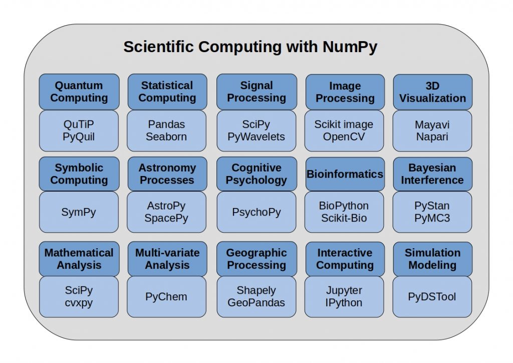
NumPy vs Pandas - The schema shows Scientific Computing with NumPy over science disciplines
NumPy vs Pandas – Scientific Computing with NumPy

NumPy was developed specifically for scientific calculations and forms the basis for many specific frameworks and libraries.

The elementary NumPy data structure

The core functionality of NumPy is based on the “ndarray” data structure.
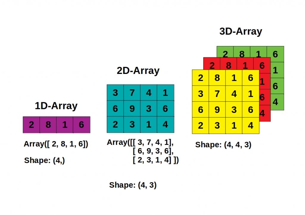
The schema shows NumPys fundamental data structure
NumPy vs Pandas – NumPys fundamental data structure

Such an array can only hold elements of the same data type and always consists of a pointer to a contiguous memory area together with the metadata describing the data stored in it. This allows processes to access them very efficiently and manipulate them as desired.
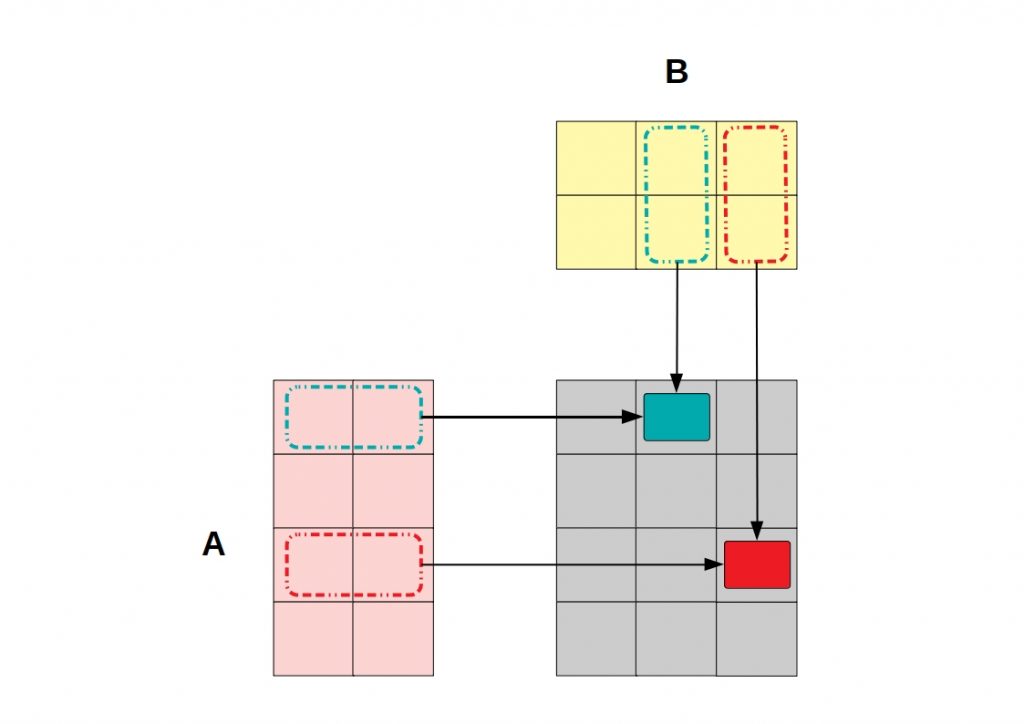
The schema shows how NumPys fundamental data structure could be manipulate
NumPy vs Pandas – NumPys data structure is manipulable

Thus, the shape can be changed via so-called reshaping, smaller subarrays can be created within a given larger array, arrays can be split, or merged.

What is Pandas?

Pandas is an open source library for data analysis and manipulation in Python. Already released in 2008 by Wes McKinney and written in Python, Cython and in C. Pandas are used in almost all areas and find worldwide appeal in all industries.
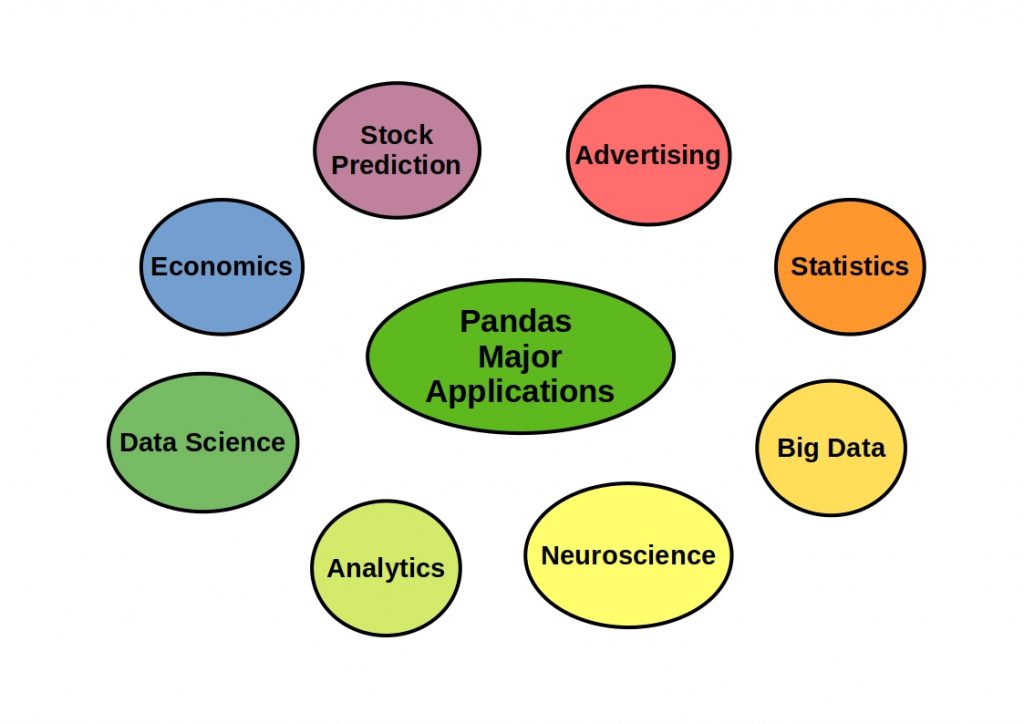
The schema shows Pandas major applications
NumPy vs Pandas – Pandas Major Applications

The name Pandas is derived from Panel Data.
Its strength lies in the processing and analysis of tabular data and time series.
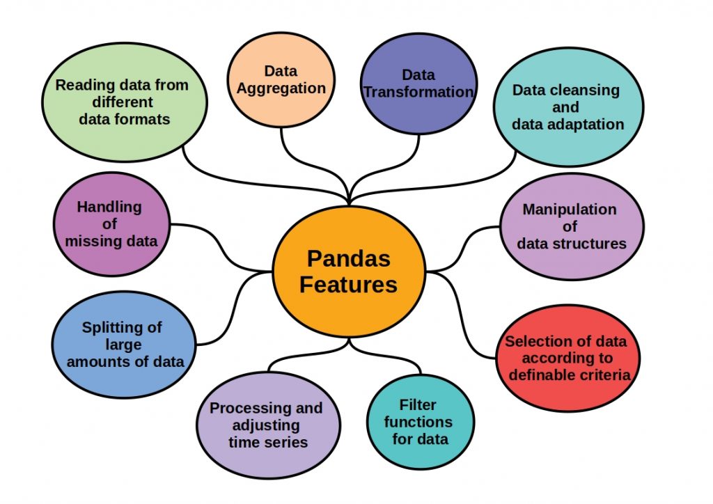
The schema shows Pandas major features
NumPy vs Pandas – Pandas Features

Especially in the pre-processing of data, pandas offers a lot of operations. In addition to high-performance filter functions, very large data volumes with over 500 thousand rows can be transformed, manipulated, aggregated and cleaned.

Pandas fundamental data structures

As a basis for the individual functions and tools that Pandas provides, the library defines its own data objects. These objects can be one, two, or even three-dimensional.

The one-dimensional series object can take up different data types in contrast to NumPys ndarrays and corresponds to a data structure with two arrays. One array as index and one array holding the actual data.

The two-dimensional DataFrame object contains an ordered collection of columns. Here, each column can consist of different data types and each value is unique by a row index and a column index.
The eponymous Panel object is then a three-dimensional dataset consisting of dataframes. These objects can be divided into major axes, which are the index rows of each DataFrame, and minor axes, which are the columns of each of the DataFrames.

NumPy vs Pandas – Conclusion

Both libraries have their similarities, which are due to the fact that Pandas is based on NumPy, but is it an either or question? No, clearly not. Pandas is based on NumPy, but adds so many individual features to its functionality that there is a clear justification for their parallel existence. They simply serve different purposes and should be used for both.


One of the main differences between the two open source libraries is the data structure used. Pandas allows analysis and manipulation on a tabular form while NumPy works mainly with numerical data in arrays whose objects can have up to n dimensions. These data forms are easily convertible among themselves via an interface.

Pandas is more performant especially with very large data sets (500K rows and more). This makes data preprocessing and reading from external data sources easier to perform with Pandas and can then be transferred as a NumPy array into complex machine learning or deep learning algorithms. If you want to know more about machine learning methods and their fields of application, take a look at this article from us.
TensorFlow or Theano?

TensorFlow or Theano – TensorFlow, along with PyTorch, is currently the best known and most widely used machine learning framework. However, the choice of tool should never depend on one’s own preferences, but should be adapted to the data to be examined. Especially in the Big data area, this can prevent a decisive loss of performance. It is therefore also worthwhile to look off the beaten track and to look at other frameworks and libraries in addition to the top dogs.
Theano is one such open source Python library. In the following article, we will introduce both tools and explain the differences.

What is Tensorflow?

The open source framework TensorFlow is the direct successor of Google’s first deep learning tool DistBelief and primarily also forms the basis for neural networks in the environment of language and image processing tasks. With TensorFlow, own models can be developed and processed, but also pre-trained models can be accessed. TF runs on a variety of platforms and is implemented in Python and C++.

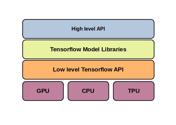
TensorFlow vs Theano - This figure shows the hierarchy of the TensorFlow framework.
Hierarchy of TensorFlow toolkits

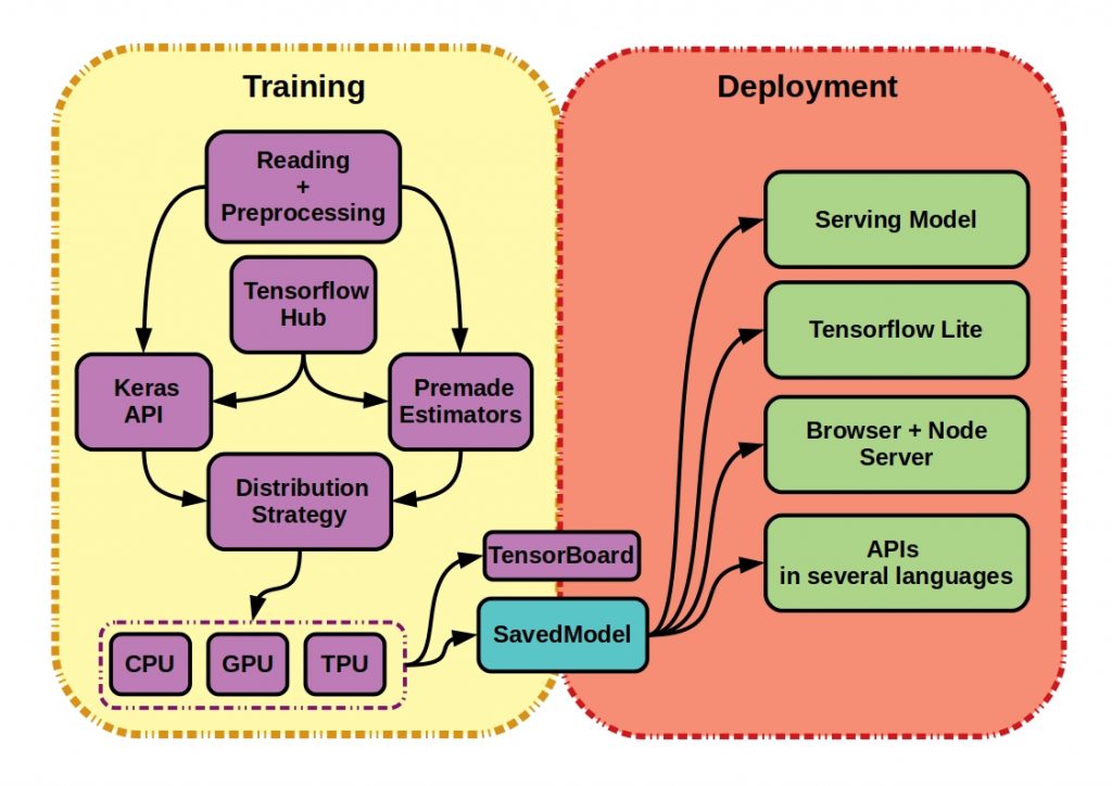
TF offers low-level APIs for CPU, GPU or TPU. In this way, the hardware resources can be optimally adapted to the process through dynamic allocations.
In addition to the low level APIs, there are also various high level APIs, such as Keras, one of the best known and most frequently used. If you want to know more about Keras, check out our article on the topic.

Framework Architecture

Mainly, the TensorFlow framework can be divided into the components needed for training, where the models are prepared for field use, and for the final deployment, for example on mobile and IoT devices with TensorFlowLite. To simplify the training, TensorFlow offers the developer some useful services besides the already mentioned dynamic allocation. For example, a premade estimator offers a high-level representation of a complete model.Via the TensorFlow Hub, a kind of repository, even trained machine learning models can be other language bindings can be accessed.

TensorFlow vs Theano - This figure shows the structure of the TensorFlow framework.
TensorFlow or Theano – Structure of the TensorFlow Framework

The TensorBoard and StoredModels services act as connecting elements between training and deployment. TensorBoard is the visualization toolkit of TensorFlow with which the experiment results can be visualized. So here it is more of a monitoring solution for the human interface. With the StoredModels both deployment services and training services can share the models. This service thus forms a kind of intermediary, but contains a complete TensorFlow program, including all weights and calculations.

TensorFlow – Data Structure

Neural networks are represented by directed cycle-free graphs. These graphs can be represented and computed beyond the computer limits of training. A graph basically consists of nodes connected by edges. The extent to which the nodes are interconnected also usually determines the learning procedure and thus the structure of an artificial neural network.
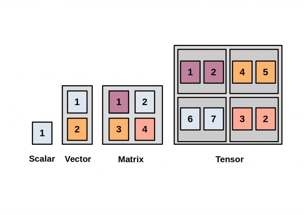
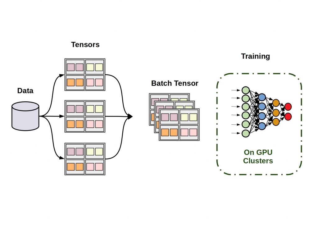
The inputs and outputs of the individual calculation steps represent multidimensional data arrays, so-called tensors.

This figure shows the basic tensor structure
Tensor Principle

The mathematical term tensor corresponds to a generalization of vectors and matrices. It is thus an elementary data structure for data representation and processing. In TensorFlow the implementation is done as multidimensional arrays . A vector thus corresponds to a one-dimensional tensor.
Additional dimensions can be added to a tensor up to infinity. Common tensor types are 3-dimensional tensors for time series, images are usually 4-dimensional, and videos are 5-dimensional tensors.

pytorch training 2
Tensors and neural networks

TensorFlow methods manipulate tensors for linear algebra operations. These processes can be executed with high performance by moving the tensor objects to the graphics card memory or tensor optimized TPUs.

TensorFlow – Training

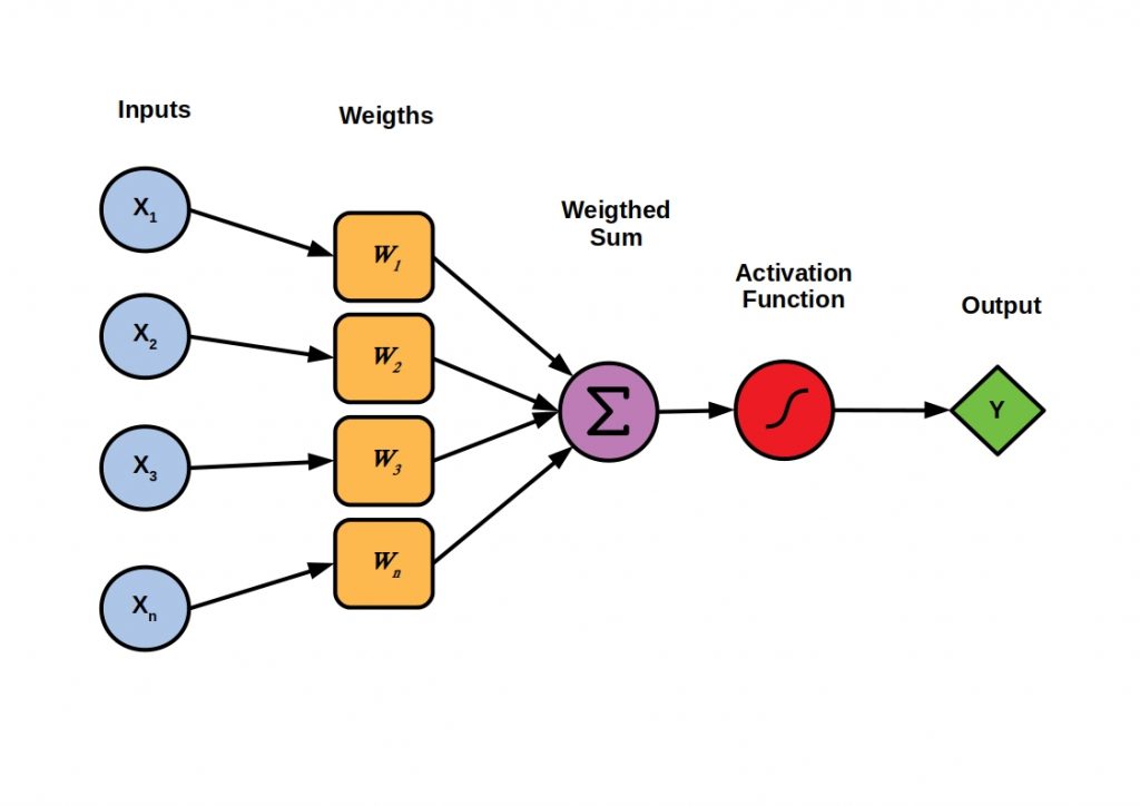
The training itself then proceeds in such a way that training data are iteratively fed into the computers and at the same time the weights within the graph are varied. The output is then approximated to a target output value. To this end, separate test data can be used to periodically verify that the training is effective for arbitrary or different input data.

 The figure shows the sequence of the training of a neural network
Training procedure

Theano – Old but Gold

Theano is an open source Python library for machine learning and neural network programming, and compiler for mathematical expression computation. It was released back in 2007 by the Montreal Institute for Learning Algorithms (MILA) at the University of Montreal.
It is particularly suitable for the definition, optimization and evaluation of mathematical expressions involving multidimensional arrays. For this purpose, Theano accesses the NumPy program library for dealing with matrices, large multidimensional arrays and vectors. First, read our article on NumPy. Here we introduce you to this elementary Python library and explain its basic data management.


Mathematical expressions are programmed and symbolized in Theano using a NumPy-like syntax.
The calculation instructions are done in C++ or CUDA code, thus very close to the machine and accordingly very efficient on CPUs or graphics processing units (GPUs).
Theano can also be used, like TensorFlow as a backend for the framework Keras. Keras thus forms an intersection for both technologies.

Graph Structure

Unlike TensorFlow, Theano focuses on supporting symbolic matrix expressions rather than tensors as a basic data type. Although all kinds of Python objects are supported, basic tensor functionality can be used with Theano, but these operations are not as optimized as with TensorFlow.

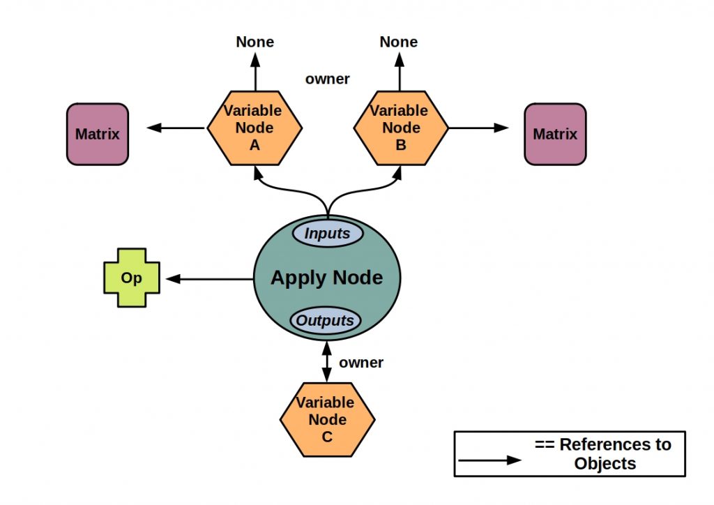
Theano performs the symbolic mathematical calculations are executed as graphs. These graphs are composed of interconnected Apply, Variable and Op nodes.

TensorFlow vs Theano - Overview structure of a Theano graph
TensorFlow or Theano – Overview structure of a Theano graph

The Op node represents a particular computation on a particular type of input that produces a particular type of output. It thus corresponds to the definition of a computation.


The centrally located Apply node represents the application of an Op to some variables, that is, the application of computations to the current data, and is used to represent a computation graph. Each op is responsible for knowing how to build an Apply node from a list of inputs and thus determines the determines the function and transformation.
An Apply node additionally consists of the input or output fields. The inputs represent the arguments of the function, and the outputs represent the return values of the function.

The Apply nodes then refer to their input and output variables, the main data structure, in the graph via their input and output fields, respectively.
These Variable Nodes are defined by various fields. The variable type, the owner, which can be None or an Apply node of which the variable is an output, the index and the variable name.

TensorFlow or Theano?

All in all, both technologies have their advantages and disadvantages. But both have their raison d’être. Here, too, the data set provides the tools.

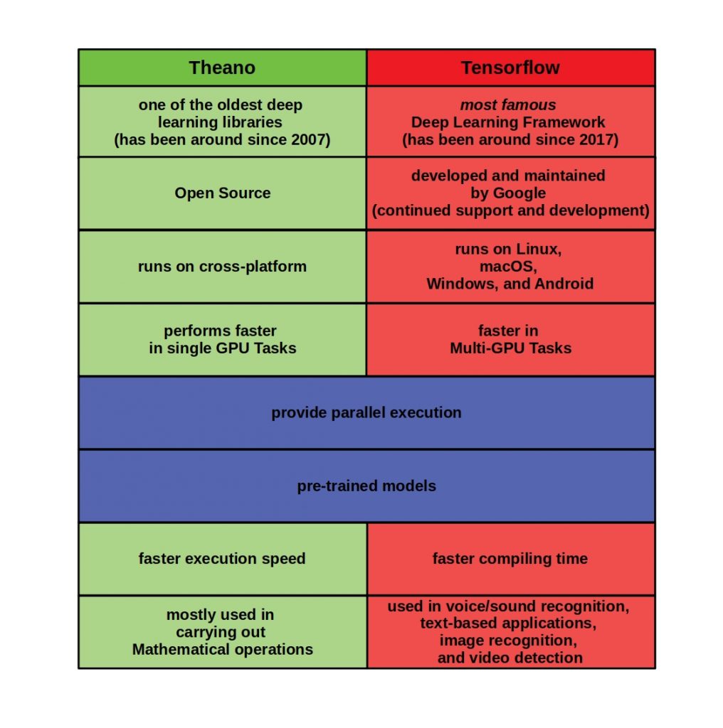
In the table below, we have listed all the important points of difference in detail.

TensorFlow vs Theano - This table compares both tools in detail.
TensorFlow or Theano – Comparision

Especially when it comes to tensor processing, as in image processing and sound recognition, TensorFlow with its optimized operations should be the first choice. Another tensor-based alternative to the Google solution is PyTorch from Facebook. In this article we compared these two tools.
Despite its age, Theano is a high-performance and modern alternative for the calculation of matrix expressions.

PyTorch vs TensorFlow – Facebook vs Google – Duel of the Giants

In recent years, the field of data science has been able to access increasingly powerful analysis methods thanks to increasingly high-performance hardware. Google’s Tensorflow has been the benchmark for editing machine learning and modeling deep learning methods. It still has the most freedom today. But a wide range of options often creates a high barrier to entry.

PyTorch vs TensorFlow – With the 2 years younger, also Python-based, open source package PyTorch, Facebook now wants to knock Tensorflow off its throne. It has been steadily gaining popularity for years due to its simplicity and features.
In this article, we will clarify what is in the package and whether it can really compete with Tensorflow.

What is PyTorch?

Pytorch is one of the most popular open source Python packages for scientific computing and neural network development/training.
It was developed by Facebook in 2016 and is based on the Torch library written in Lua. A NumPy-like tensor library that provides rich GPU support to enable accelerated neural network learning. PyTorch is also often referred to as the library of the same name. More about this in the section “Libraries”.
Tensors form the elementary data structures for PyTorch, similar to Tensorflow.

PyTorch vs TensorFlow – Tensors form the basis for both!

The mathematical term tensor corresponds to a generalization of vectors and matrices. It is thus an elementary data structure for data representation and processing. In PyTorch the implementation is done as multidimensional arrays . A vector thus corresponds to a one-dimensional tensor.

PyTorch vs TensorFlow - the figure schematically shows the principle behind tensors.
PyTorch vs TensorFlow – Tensor Principle

More dimensions can be added to a tensor up to infinity. Common types of tensors are 3 dimensional tensors for time series, images are usually 4 dimensional and videos are five dimensional tensors.

PyTorch vs TensorFlow -The figure shows the role of tensors in the training of neural networks in PyTorch.
PyTorch vs TensorFlow – Tensors and neural networks

PyTorch methods manipulate tensors for linear algebra operations. These processes can run at high performance by moving the tensor objects into the graphics card memory.

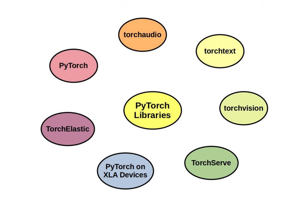
PyTorch Libraries

Pytorch offers the possibility to include specific libraries. This way the program can be kept lean and only make references to needed code.
The PyTorch library itself is an optimized tensor library for deep learning on both GPUs and CPUs.
By including another library, PyTorch can also compute on TPUs.


Depending on the data type, different libraries can be loaded, which provide optimized methods and pre-modeled prototypes for analysis. Torchaudio offers besides the usual audio transformation methods also data sets for training. With torchtext large language packages can be accessed and with torchvision images can be analyzed.

PyTorch vs TensorFlow -The figure shows all PyTorch Libraries.
PyTorch Libraries

With TorchElastic, training jobs can be managed and elatically distributed, for example, to shared capacities.

PyTorch features

Through accelerated tensor analysis via allocation to GPUs, PyTorch achieves high flexibility and high speed in Deep Learning algorithms. Beyond this, PyTorch offers through its Python base unlimited compatibilities to powerful Python libraries, such as NumPy and SciPy and to the Cython programming language. Here we have collected the most important Python open source data management and analysis libraries.


Reverse-mode auto differentiation allows developers to modify network behavior at will, without delay or overhead. This allows for essential acceleration of research iterations.
The 8-bit quantization model ensures efficient deployment on servers and edge devices, and PyTorch Mobile can be used to develop for Android and iOS environments.
Other features include named tensor, artificial neural network pruning, and parallel training of models with remote procedure call.

PyTorch can access TorchServe, an open source server from Facebook, and is fully compatible with cloud provider Amazon Web Services (AWS). If you don’t know what AWS is, read our article on the subject.

PyTorch offers a hybrid frontend as an additional feature. This offers the possibility to choose between two modes. The Eager and the Graph mode. The eager mode primarily offers usability and flexibility, while the graph mode offers better speed, optimization and functionality in a C++ runtime environment. PyTorch also allows conversion with the Hybrid frontend. This allows models to be developed in eagermode and then transferred to graph mode for production.

PyTorch has unlimited access to ONNX (Open Neural Network Exchange) compatible platforms. ONNX is an open source project jointly developed by Microsoft, Amazon, and Facebook, among others, that enables the exchange of AI models between different tools.

PyTorch vs Tensorflow

Duel of the Giants

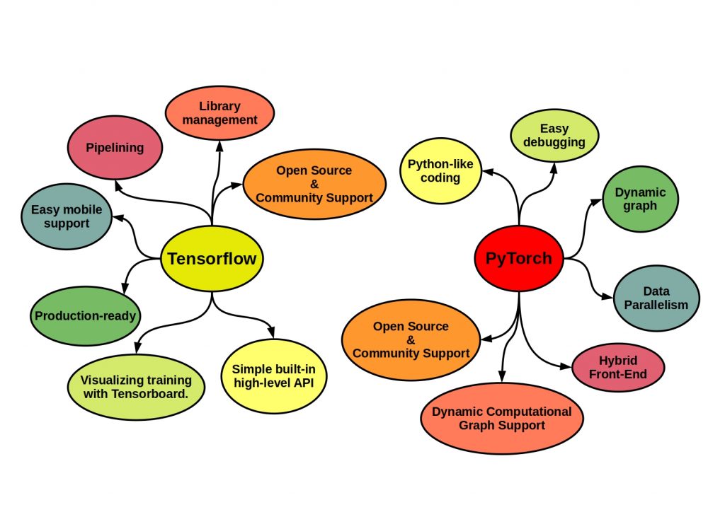
Just like the Facebook solution, Tensorflow works with the tensor data type. PyTorch scores with its simplicity and effective memory usage. Tensorflow, on the other hand, is much more scalable and thus better suited for production models. An essential difference was originally that with PyTorch the graph structure is defined during execution, while with Tensorflow it is first defined and then executed. Here, however, Tensorflow has now followed with its own eager mode. However, this is not yet fully developed at this stage.

PyTorch vs TensorFlow - The figure shows the main differences between Google's Tensorflow and Facebook's PyTorch
Tensorflow vs PyTorch

PyTorch vs Tensorflow – Who is ahead now?

It remains an exciting head-to-head race. Despite its recent development history, PyTorch has already made up a lot of ground and is interesting in an entrepreneurial context precisely because of its user-friendliness. As is often the case, however, it is not a question of which solution will come out on top, but rather of the principle that competition stimulates business. In the end, competitive pressure leads to great new innovations and exciting new tools.

Supervised vs Unsupervised vs Reinforcement Learning – The fundamental differences

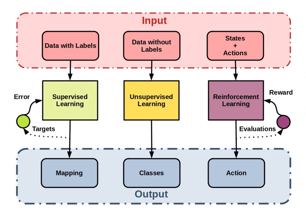
Supervised vs Unsupervised vs Reinforcement Learning – The three main categories of machine learning. Why these boundaries have been drawn and what they look like will be discussed in this article. The knowledge about this is an elementary part to understand machine learning correctly and to be able to apply it to data in a meaningful way.

This figure contrasts Supervised vs Unsupervised vs Reinforcement Learning.
Supervised vs Unsupervised vs Reinforcement Learning – Overview

Supervised vs Unsupervised vs Reinforcement Learning – Machine Learning Categories

Machine learning is a branch of artificial intelligence. While AI deals with the functioning of artificial intelligence and compares it with the functioning of the human brain, machine learning is a collection of mathematical methods of pattern recognition. If you want to know more about the differences between Machine Learning, AI and Deep Learning, read our article on the subject. IT systems should be given the ability to automatically learn from experience and improve. Algorithms play a central role here. These can be classified into different learning categories.

In the following figures the three main categories of machine learning methods are shown.

This figure shows Supervised vs Unsupervised vs Reinforcement Learning in the machine learning context.
Supervised vs Unsupervised vs Reinforcement Learning – Machine Learning Context

In the meantime, there are many more categories, some of which are hybrids of the individual main categories. One example is semi-supervised learning. This is certainly also a major machine learning topic, but has been left out for the time being for the sake of simplicity.

What is supervised learning?

In supervised learning, the machine learning algorithm iteratively learns the dependencies between data points. The output to be learned is specified in advance and the learning process is supervised by matching the predictions. How the The optimized algorithm is to apply the learned patterns to unknown data to make predictions.

Supervised vs Unsupervised vs Reinforcement Learning - This figure shows the basic principle of supervised learning.
Supervised vs Unsupervised vs Reinforcement Learning – Supervised Learning

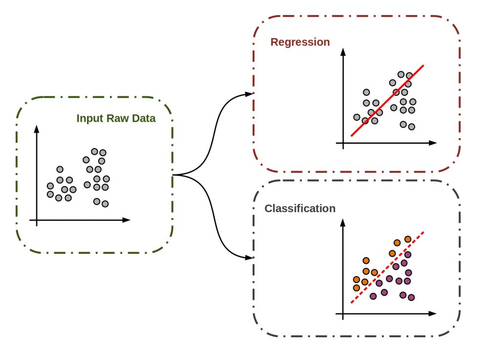
Supervised learning methods can be applied to regression, i.e., prediction, or trend prediction, as well as classification problems.

What is supervised classification?

In classification, abstract classes are formed in order to delimit and order data in a meaningful way. For this purpose, objects are obtained on the basis of certain similar characteristics and structured among each other.

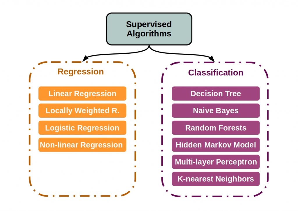
Decision trees can be used as prediction models to create a hierarchical structure, or the feature values can be assigned as class labels and in the form of a vector.

In the following figure the most important supervised classification algorithms are listed.

Supervised vs Unsupervised vs Reinforcement Learning - This figure shows the main algorithms of supervised learning.
Supervised vs Unsupervised vs Reinforcement Learning – Main Algorithms of Supervised Learning.

What is supervised regression?

On the other hand, supervised regression algorithms can be used to make predictions and infer causal relationships between independent and dependent variables.
For example, linear regression can be used to fit the data to a straight line or, conversely, to fit a line to the data object.
We have discussed the exact process of linear regression here in this article.

What is unsupervised learning?

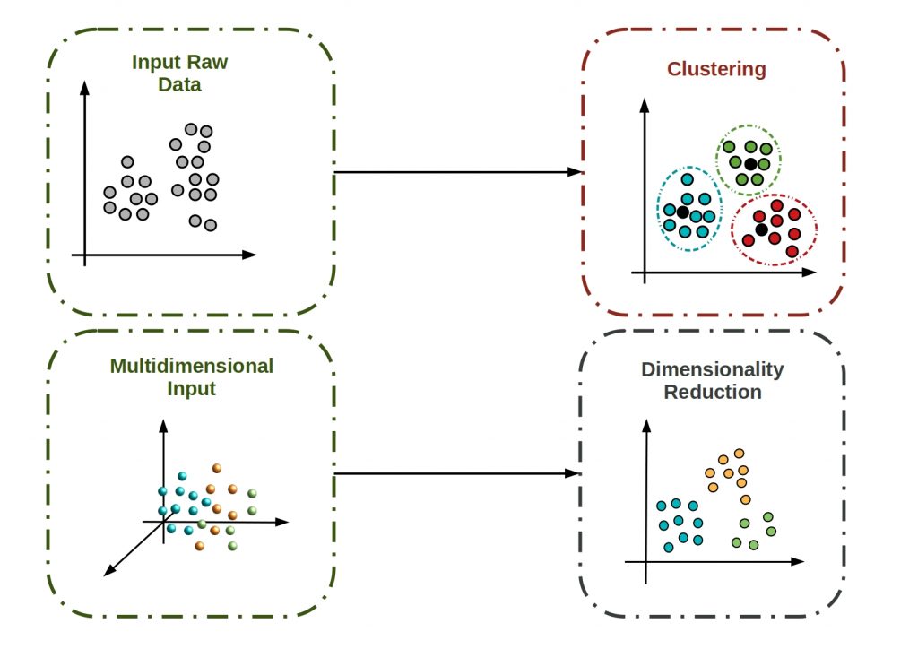
In unsupervised learning, patterns are determined in data without initial patterns and relationships being known.
Especially in complex tasks, these methods can be useful to find solutions that would hardly be solvable by hand. An example is autonomous driving, or large biochemical systems with many interactions.
One key to success is a huge data set. The more data available, the more accurate models can be created.

Supervised vs Unsupervised vs Reinforcement Learning - This figure shows the basic principle of unsupervised learning.
Supervised vs Unsupervised vs Reinforcement Learning – Unsupervised Learning

In unsupervised machine learning methods, two basic principles, which also classify the algorithms used, can be distinguished. The clustering and the dimensional reduction.

What is unsupervised clustering?

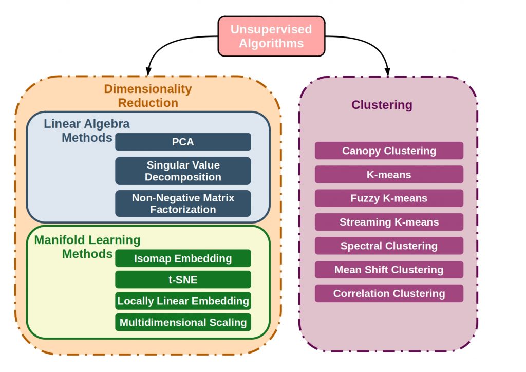
The main goal of unsupervised clustering is to create collections of data elements that are similar to each other, but dissimilar to elements in other clusters. The figure below shows some of the main clustering algorithms.

Supervised vs Unsupervised vs Reinforcement Learning - This figure shows the main algorithms of unsupervised learning.
Supervised vs Unsupervised vs Reinforcement Learning – Main algorithms of unsupervised learning.

The clustering algorithms differ primarily in the cluster creation process, but also in the definition of such clusters. Thus, the relationships between clusters can also be used and hierarchical relationships can be explored.

What is unsupervised dimensional reduction?

With a high number of features, high dimensional relations can be translated low dimensional with these transformation methods. The goal is to keep the loss of information as small as possible.
The reduction methods can be divided into two main categories: Methods from linear algebra and from manifold learning.

Manifold learning is an approach to nonlinear dimensionality reduction. Algorithms for this task are based on the idea that they can learn the dimensionality of the data without a given classification and project it in a low-dimensional way.
For example, from the field of linear algebra, matrix factorization methods can be used for dimensionality reduction.

What is reinforcement learning?

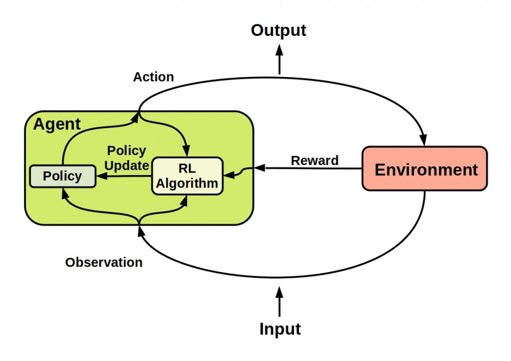
In reinforcement learning, a program, a so-called agent, should independently develop a strategy to perform actions in an environment. For this purpose, positive or negative reinforcements are conveyed, which describe the interaction interactions of the agent with the environment. In other words, immediate feedback on an executed task. The program should maximize rewards or minimize punishments. The environment is a kind of simulation scenario that the agent has to explore.
The following figure describes the interactions of all components of a reinforcement learning process.

Supervised vs Unsupervised vs Reinforcement Learning - This figure shows the main principle of reinforcement learning.
Supervised vs Unsupervised vs Reinforcement Learning – Main principle of reinforcement learning.

There are two basic types of reinforcement learning.
Namely, whether the environment is model-based or not.
In model-based RL, the agent uses predictions of the environment response during learning or action.
If no model is available, the data is generated by trial and error.

Things you need to know when you start using Apache Spark

Apache Spark Streaming – Every company produces several million pieces of data every day. Properly analyzed, this information can be used to derive valuable business strategies and increase productivity.
Until now, this data was consumed and stored in a persistent. Even today, this is an important step in order to be able to perform analyses on historical data at a later date. Often, however, analysis results are desired in real time. Be it only reference values that have been exceeded.


So-called data streams, i.e. data that is continuously generated from thousands of data sources, can already be consumed before they end up in a persistence, without the flow rate being significantly reduced. It is even possible to train neural networks using such a stream.


In this article, we’ll tell you why you shouldn’t miss out on Apache Spark and Apache Spark Streaming if you’re planning to integrate stream processing in your organization.

What is Apache Spark?


Apache Spark has become one of the most important and performant unified data analytics on the market today. The framework provides a total solution of data processing and AI integration. This allows companies to easily develop performant data pipelines and train AI methods using massive data streams.


Apache Spark combines several partially interdependent components. So can be deployed in a modular fashion to a certain extent.
Spark can run in its standalone cluster mode, on EC2, on Hadoop YARN, on Mesos or on Kubernetes.
The data here can come from streaming sources, such as Kafka, as well as static data sources. So far, the programming languages Java, Scala, Python and R are supported. These are currently the most commonly used languages across all scientific disciplines for implementing data analysis methods.

What does a Spark cluster look like?

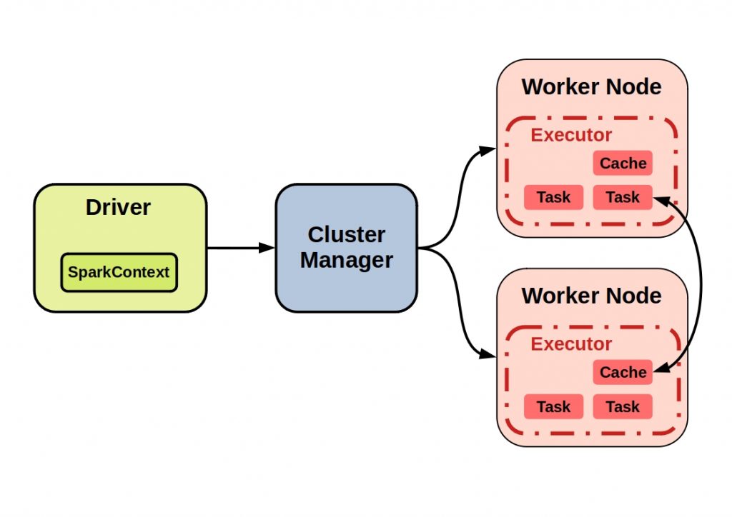
Spark applications run as independent sets of processes on a cluster.The coordinator of a Spark program on a cluster is the so-called SparkContext object. This controls the individual Spark applications as they run as independent processes.
The Coordinator then connects to the Central Element, a Cluster Manager, which then allocates resources to the individual applications.
The figure below shows an example of a typical Spark cluster with all its components.

The figure  shows an example of a typical Spark cluster with all its components.
Overview Apache Spark Cluster

The actual calculations and data storage then take place on the nodes. These processes, also called executors, then execute tasks and hold the data in memory or disk space. The cache can then be accessed by another node.

Apache sparks underlying technology – The key to high Performance

Spark Core is the underlying unified computing engine on which all Spark functions are built. It enables parallel processing even for large datasets and thus ensures very high-performance processes.
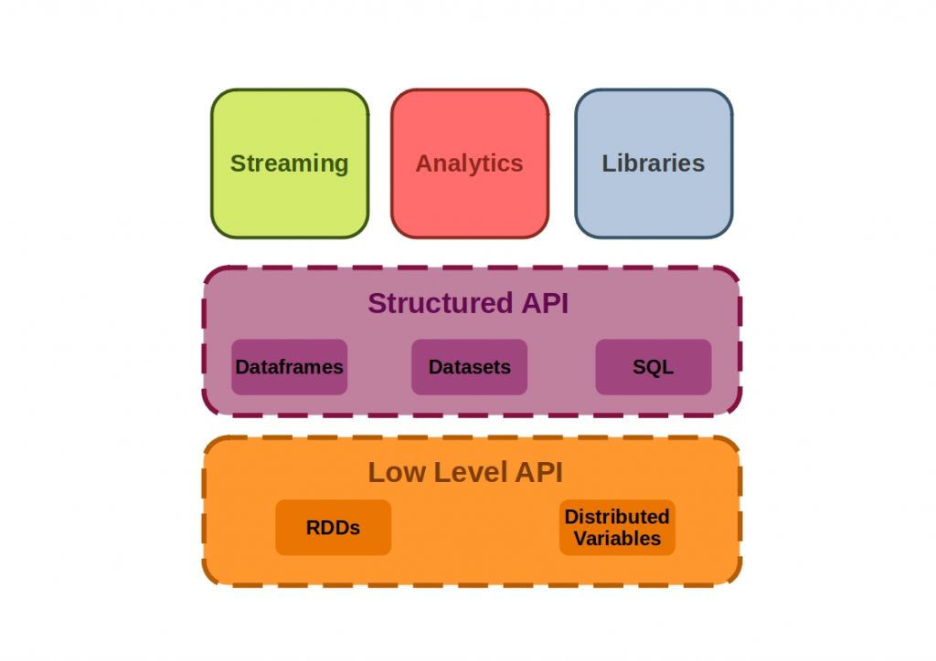
The following figure shows how the Apache Spark Core APIs are composed.

The  figure shows how the Apache Spark Core APIs are composed.
Apache Spark Core APIs

The core API consists of low level APIs, where object manipulation via Resilient Distributed Datasets (RDDs) takes place and structured APIs, where all data types are manipulated and batch or streaming jobs take place.

How do the individual Apache Spark APIs work?

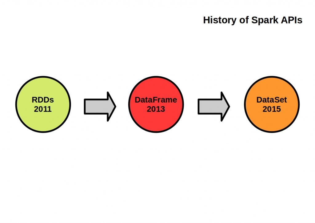
In order to properly understand the API structure, its components must be placed in a historical context.

The figure shows the development history of the Apache Spark APIs.
Development history of the Apache Spark APIs

What is the RDD API?

The RDD (Resilient Distributed Dataset) API has been implemented since the first Spark release and is based on the Scala collections API.
RDDs are a set of Java or Scala objects that represent data and thus are the building blocks of Spark. They excel in being compile-time type-safe and inert.

All higher level APIs can be decomposed into RDDs. Various transformations can be performed in parallel using this API. Each of them defines an operation to be executed, which is invoked by calling an action method and creates a new RDD. This then represents the transformed data.

What is the Dataframe API?

The Dataframe API introduces a higher level abstraction. Spark dataframes correspond to the Pandas dataframes structure. They are built on top of RDDs and represent two-dimensional data and a schema. It contains an ordered collection of columns and each different column can consist of different data types. Each value is unique by a row and a column index.


When data is transferred between nodes, only the data is transferred. The metadata is managed in a schema registry separate from spark. This has significantly improved the performance and scalability of Spark.
The API is suitable for creating a relational query plan. Thus, manipulation of data can now be done using a query language.

What is the Dataset API?

When working with dataframes, compile-time type safety is lost. This is a strength of the RDD API. The Dataset-API was created to combine the advantages of both APIs. It is thus the second most important Spark API next to the RDD API.


The basis of this API are integrated encoders, which are responsible for the conversion between JVM objects and the internal Spark SQL representation.

What components does Apache Spark consist of?

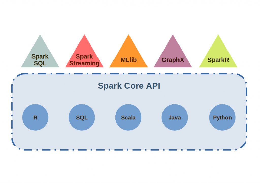
Spark is modularly extensible through the use of components. Spark includes libraries for various tasks ranging from SQL to streaming and machine learning. All components are based on the Spark Core, the foundation for parallel and distributed processing of large data sets. How this API looks in detail and what makes it so performant, we will explain later.
The following figure lists the individual Apache Spark components.

In the figure, the ecosystem of Apache Spark is shown with all the major components.
Apache Spark Ecosystem

Apache Spark Spark SQL

With this component RDDs are converted into the so-called data frames, i.e. provided with metadata information.
The whole thing is done by a catalyst optimizer, which executes an execution plan in the form of a tree.

Apache Spark GraphX

This framework can be used to perform high-performance calculations on graphs. These operations can run in parallel.

Apache Spark MLlib/SparkML

With the MLlib component, machine learning pipelines can be constructed very easily. For this purpose, ready-made models and common machine learning algorithms (classification, regression, clustering …) can be used. Thus, data identification, feature extraction and transformation are combined in a unified framework.

Apache Spark Streaming

Apache Spark Streaming enables and controls the processing of data streams. However, Apache Spark Streaming can also process data from static data sources.
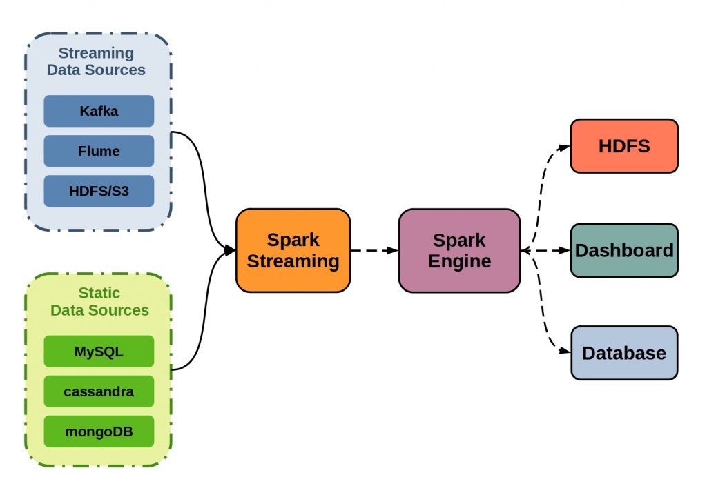
In the case of datastreaming, input stream goes from a streaming data source, such as Kafka, Flume or HDFS, into Apache Spark Streaming.
There, it is broken into batches and fed into the Spark engine for parallel processing. The final results can then be output to HDFS databases and dashboards.
The following figure illustrates the principle of Apache Spark Streaming.

The figure illustrates the principle of Apache Spark Streaming.
Principle of Apache Spark Streaming

All components can consume directly from the stream via Apache Spark Streaming. This component takes a crucial role here. It coordinates the requests via sliding window operations and regulates the data flow. Since all components are based on the Spark Core API, absolute compatibility is guaranteed. Especially in the Big Data area, this can deliver a decisive performance bonus.
PCA vs Linear Regression – Therefore you should know the differences

PCA vs Linear Regression – Two statistical methods that run very similarly. However, they differ in one important respect. What the two methods actually are and what this difference is, we explain to you in the following article.

What is a PCA?

Principal Component Analysis (PCA) is a multivariate statistical method for structuring or simplifying a large data set. The main goal here is the discovery of relationships in 2 or 3 dimensional domain.
This method enjoys great popularity in almost all scientific disciplines and is mostly used when variables are highly correlated.


However, PCA is only a reliable method if the data are at least interval scaled and approximately normally distributed.
Although the variables are adjusted to avoid redundant effects, the error and residual variance of the data are not taken into account.

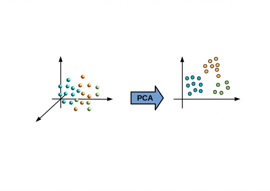
The following figure shows the basic principle of a PCA. High dimensional data relationships should be represented in a low dimensional way, with as little loss of information as possible.

PCA vs Linear Regression - Figure shows the basic principle of a PCA. High dimensional data relationships should be represented in a low dimensional way, with as little loss of information as possible.
PCA vs Linear Regression – Basic principle of a PCA

The key point of PCA is dimensional reduction. It is to extract the most important features of a data set by reducing the total number of measured variables with a large proportion of the variance of all variables.
This reduction is done mathematically using linear combinations.
What are linear combinations?

PCA works in a purely exploratory way, searching the data for a linear pattern that best describes the data set.
These linear combinations can best be thought of as straight lines between variable values.
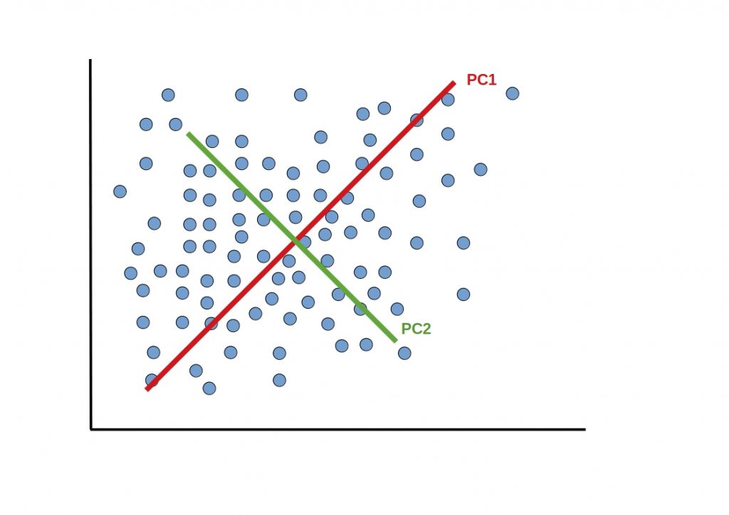
In the figure below, the linear combinations have been applied to a data set.

PCA vs Linear Regression -In this scheme the linear combinations have been applied to a data set
Linear combinations

How does the algorithm work?

In the principal component analysis procedure, a set of fully uncorrelated principal components are first generated.
These contain the main changes in the data and are also known as latent variables, factors or eigenvectors.
The number of extracted components is given here by the data.

The first principal component is formed by minimizing the sum of squared variances of all variables.
During extraction, the variance component is maximized over all variables.
Then, the remaining variance is gradually resolved by the second component until the total variance of all data is explained by the principal components.

The first factor always points in the direction of the maximum variance in the data.
The second factor must be perpendicular to it and explain the next largest variance

PCA vs Linear Regression – How do they Differ?

We have studied the PCA and how it works in great detail. But what are the differences to linear regression?

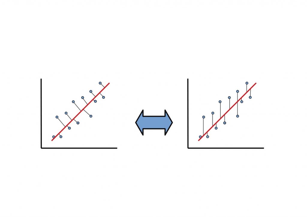
In the following illustration the main difference is set up against each other.

PCA vs Linear Regression -  The figure shows the main difference between the two methods. The minimization of the error squares to the straight line.
PCA vs Linear Regression – Minimization of the Error Squares to the Straight Line

With PCA, the error squares are minimized perpendicular to the straight line, so it is an orthogonal regression. In linear regression, the error squares are minimized in the y-direction.

Thus, linear regression is more about finding a straight line that best fits the data, depending on the internal data relationships.
Principal component analysis uses an orthogonal transformation to form the principal components, or linear combinations of the variables.

So this difference between the two techniques only becomes apparent when the data are not completely independent, but there is a correlation.

If you want to know more about machine learning methods and how they work, check out our article on the t-SNE algorithm.

t-SNE – Great Machine Learning Algorithm for Visualization of High-Dimensional Datasets

The machine learning algorithm t-Distributed Stochastic Neighborhood Embedding, also abbreviated as t-SNE, can be used to visualize high-dimensional datasets. Each high-dimensional information of a
data point is reduced to a low-dimensional representation. However, the information about existing neighborhoods should be preserved.

So this technique is another tool you can use to create meaningful groups in unordered data collections based on the unifying data properties. If you don’t know what cluster algorithms are, check out this article. Here we present 5 machine learning methods that you should know.
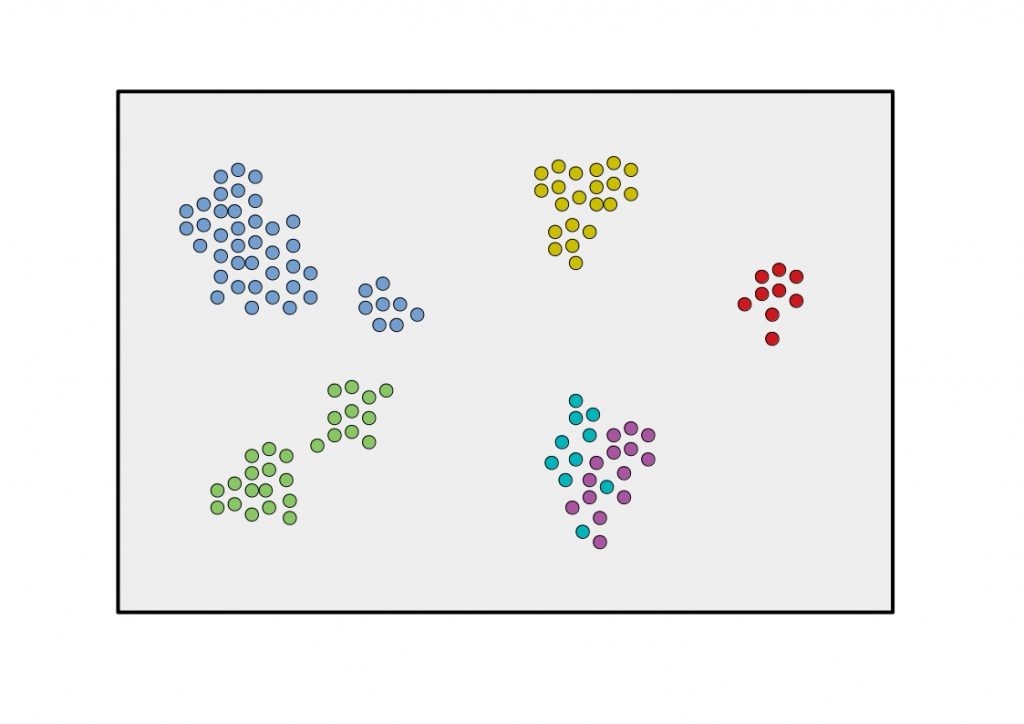
As shown in the following figure, the data should be represented grouped in 2-dimensional space.

The figure shows the data clusters generated by t-Distributed Stochastic Neighborhood Embedding (T-SNE) in 2-dimensional space.
Data clusters generated by t-Distributed Stochastic Neighborhood Embedding (T-SNE)

But how does the algorithm work and what are its strengths? In order to understand its function, we need to look at the origin of the technology.

What is the Stochastic Neighbor Embedding (SNE) Algorithm?

The basis of the t-Distributed Stochastic Neighborhood Embedding algorithm is originally the Stochastic Neighbor Embedding (SNE) algorithm. This converts high-dimensional Euclidean distances into similarity probabilities between individual data points.
The probability with which an object occurs next to a potential neighbor must be calculated.
The dissimilarities between two high-dimensional data points can be explained with a distance matrix, corresponding to the squared Euclidean distance.
A conditional probability is calculated for the low-dimensional correspondence.
This determines the similarity of the two data points on the low-dimensional map.

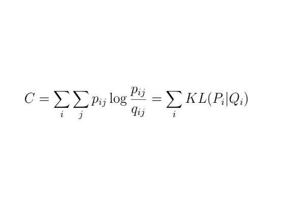
In order to achieve the closest possible correspondence between the two distributions pij and
qij, a Kullback-Leibler divergence (KL) over all neighbors of each data point is computed as a cost function C. Large costs are incurred for distant data points.

t-Distributed Stochastic Neighborhood Embedding: minimized cost function: sum of the Kullback-Leibler divergences between the original and the induced distribution over the neighbors of an object.
Minimized Cost function: sum of the Kullback-Leibler divergences between the original and the induced distribution over the neighbors of an object.

A gradient descent method is used to optimize the cost function. However, this optimization method converges very slowly. In addition, a so-called crowding problem arises.

If a high dimensional data set is linearly approximated in a small scale, then it cannot be reduced to a lower dimension with a local scaling algo-
rithm to a lower dimension.

What makes the t-Distributed Stochastic Neighborhood Embedding (t-SNE) Algorithmt work?

The t-Distributed Stochastic Neighbor
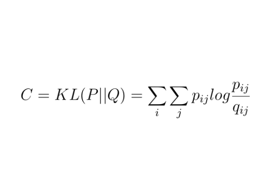
Embedding (t-SNE) algorithm starts here. On the one hand, a simplified symmetric cost function is used.

The figure shows the simplified symmetric cost function used in t-Distributed Stochastic Neighborhood Embedding.
t-SNE: simplified symmetric cost function

Here, only one KL is minimized over a common probability distribution of all
high, and low dimensional data is minimized.

On the other hand, the similarity of the low-dimensional data points is computed with a Student’s t-distribution and a degree of freedom of one. This can be optimized quickly and is stable to the crowding problem.
stable against the crowding problem.

AI vs Machine Learning vs Deep Learning – It’s almost harder to understand all the acronyms around AI than the technology itself.

It’s almost harder to understand all the acronyms around Artificial Intelligence (AI) than the technology itself.
AI vs Machine Learning vs Deep Learning – These terms are often carelessly mixed together. But what are actually the differences? In this article, we will introduce you to all Three fields, because even though there is overlap, they differ.
It should be important for you to know these differences, as each discipline describes different stages of a data analysis pipeline.

AI vs Machine Learning vs Deep Learning

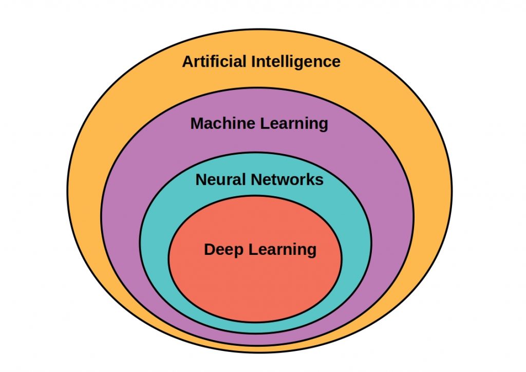
In the following figure, we have schematically shown you the individual fields in their context. As you can see, the individual disciplines surround each other and form an onion-like layered model.

Schematic representation of ai vs Machine Learning vs  Deep Learning.
AI vs Machine Learning vs Deep Learning – Contextual representation of the AI disciplines

The figure clearly shows that there are relationships between individual disciplines. AI is to be understood as a generic term and thus includes the other fields. The deeper you go in the model, the more specific the tasks become. In the following, we will follow this representation and work our way from the outside to the inside.

Artificial intelligence

All disciplines are encompassed by the term AI. It is a science that explores ways to build intelligent programs and machines that can perceive, reason, act, and solve problems creatively. To this end, it attempts to model how the human brain works.
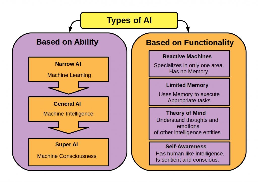
The following figure shows that AI can basically be divided into two categories.

AI vs Machine Learning vs Deep Learning
Ability and functionally based AI types simply explained
Types of AI

Classification is about measuring the performance of AI based on how well it is able to replicate the human-like brain. In the Based on Functionality category, AI is classified based on how well it matches the human way of thinking. In the second category, it is evaluated based on human intelligence. Within these categories, there are still some subgroups that correspond to an index.

AI vs Machine Learning

So what is the first subcategory Machine Learning and how does it differ from AI?
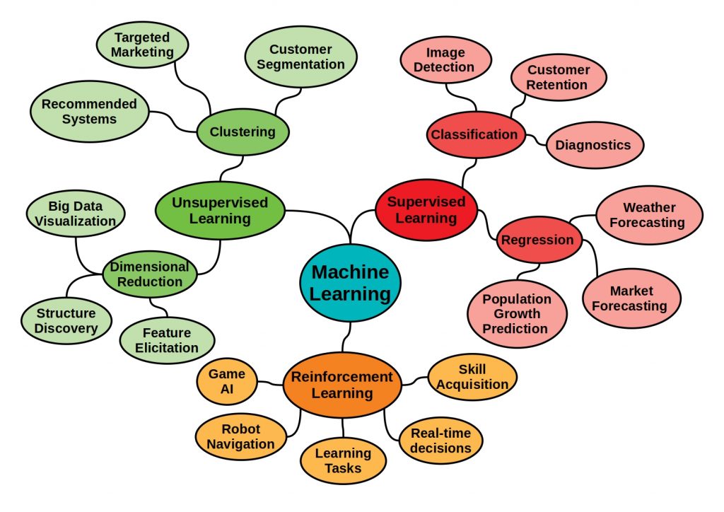
While AI deals with the functioning of artificial intelligence and compares them with the functioning of the human brain, machine learning is a collection of mathematical methods of pattern recognition. It is about how a system is given the ability to automatically learn and improve from experience. Various algorithms (e.g., neural networks) are used for this purpose. In the following scheme, the broad machine learning field is presented in a categorized way.

AI vs Machine Learning vs Deep Learning
Presentation of all basic machine learning parts
Definition Machine Learning

In machine learning, algorithms are used to build statistical models based on training data. Roughly, these algorithms can be divided into three main learning techniques. While in supervised learning the result is predetermined by a cleanly labeled data set, unsupervised learning is completely self-organized. Here the patterns are to be explored independently.
In reinforcement learning, utility functions are to be independently approximated based on rewards received.

Machine Learning vs Deep Learning/ Deep Neural Learning

Deep learning is a subfield of machine learning similar to machine learning in Ai. Here, multilayer neural networks are used to analyze various factors in large amounts of data. These networks are similar to the human neural system. If you want to know more about this structure, read our article on perceptrons, the smallest unit of a neural network.
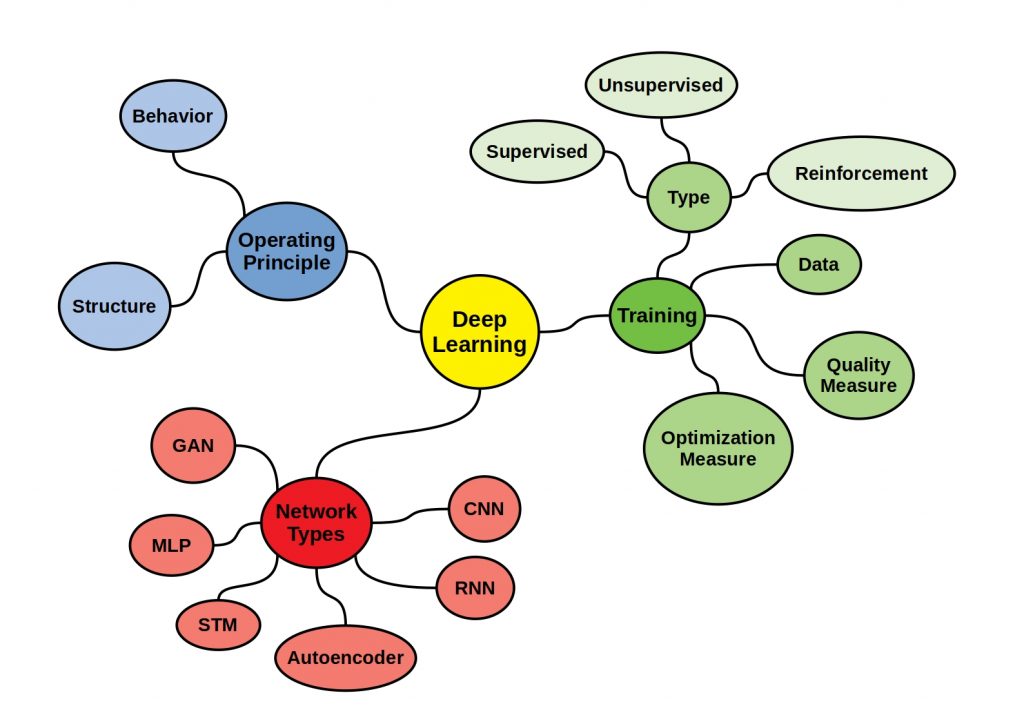
Optimization of neural weights, unlike machine learning, can be done using powerful GPUs. Pure machine learning is best used on structured data sets, while for unstructured data you should opt for deep learning. In the following graphic, we have summarized the main factors that make up deep learning. For the network types autoencoder and CNN we provide more detailed articles.

Representation of all basic deep learning components
AI vs Machine Learning vs Deep Learning
Definition Deep Learning

H2O AI – That’s why it’s so great

There is a lot of Big Data software available now. One of them that you should definitely know about is the H2O AI Machine Learning solution.

With this open-source application you can implement algorithms from the fields of statistics, data mining and machine learning. The H2O AI Engine is based on the distributed file system Hadoop and is therefore more performant than other analysis tools. Your machine learning methods can thus be used as
parallelized methods.

Software Stack

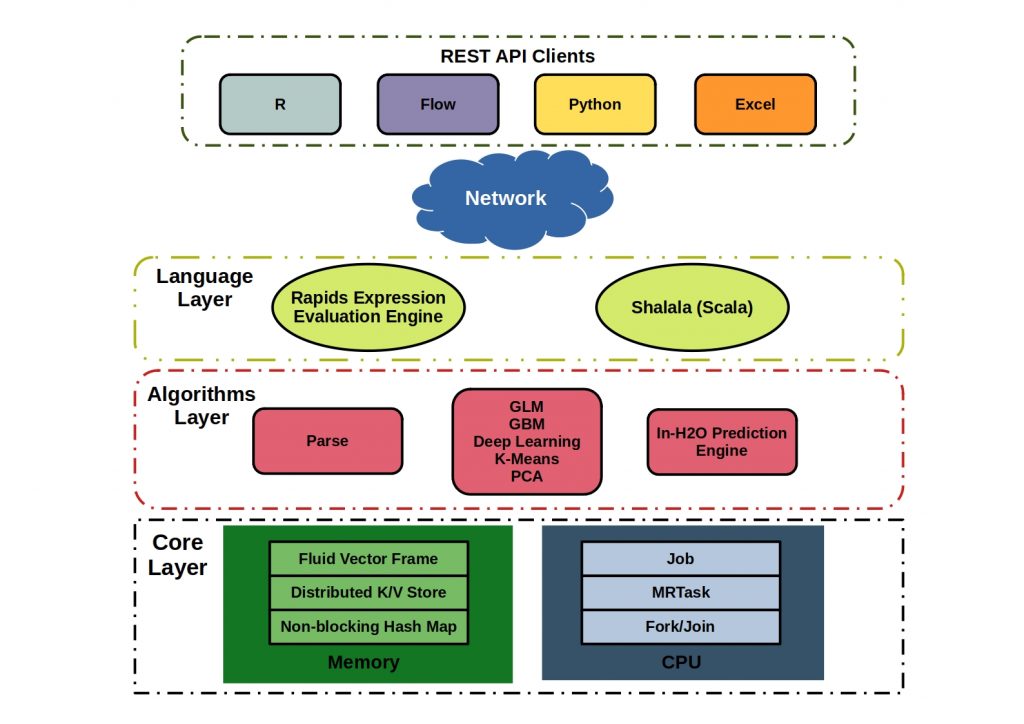
They can program their algorithms in R, Python and Java and thus in the most important mathematical programming languages. H2O provides a REST interface to Python, R, JSON and Excel. Additionally, you can access H2O directly with Hadoop and Apache Spark. This makes integration into your data science workflow much easier. You already get approximate results while running the algorithms. A graphical web browser UI helps you to better analyze the processes and perform targeted optimizations.

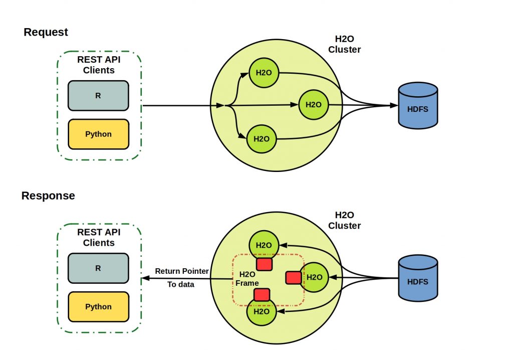
How Clients Interacts with H2O AI

You can interact with H2O via clients using various interfaces. It is important for you to know that the data is usually not held in memory. They are localized in a H2O cluster and you only get a pointer to the data when you make a request.

How Clients Interacts with H2O AI
H2O Interaction flow

H2O Frame

The basic unit of data storage accessible to you is the H2O Frame. This corresponds to a two-dimensional, resizable and potentially heterogeneous data point. This tabular data structure also contains labeled axes.

H2O Cluster

Your H2O cluster consists of one or more nodes. A node corresponds to a JVM process and this process consists of three layers.

H2O Machine Learning Software Structure
H2O Software Stack

H2O Machine Learning Components

Language Layer

The R evaluation layer is a slave to the REST client front-end and in the Scala layer you can write native programs and algorithms. You can then use these with H2O Machine learning.

Algorithms Layer

This layer is where your algorithms are applied. You can run statistical methods, data import and machine learning here.

Core Layer

In this layer you handle the resource management. You can manage both the memory and the CPU processing capacity.

5 Clustering Algorithms Data Scientists need to know – The key is always to understand the basic approach of any algorithm you want to use

As a data scientist, you have several basic tools at your disposal, which you can also apply in combination to a data set. Here we present some clustering algorithms that you should definitely know and use

In times of Big Data, not only the sheer number of data increases, but also the relationships between them. More and more complex dependencies are formed. This makes it all the more difficult to recognize these similar properties and to assign the data to so-called clusters in a way that can be evaluated.

You have certainly heard of these algorithms and maybe used one or the other, but do you really know what clustering algorithms are?

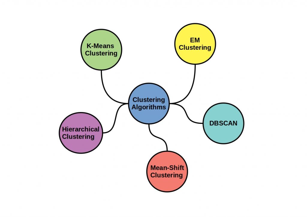
What are clustering algorithms?

So let’s first clarify what these algorithms are in the first place. The goal is clear: You want to identify similar properties between individual data points in a data set and group them in a meaningful way. These properties are often high-dimensional.

With the help of cluster analysis, you want to reduce this high-dimensional information to a low-dimensional dependency. So, for example, a representation in 2D space. Clustering is an unsupervised machine learning technique and in the end you classify the data points by using algorithms.

The approach to clustering differs from technique to technique. All have their advantages and disadvantages, so it makes sense to try several on one set of data, or apply them in combination. Below we will introduce you to some popular clustering methods and explain their grouping approach.

This picture shows schematically popular Clustering Machine Learning Algorithms you should know as a data scientist
Clustering Machine Learning Algorithms – Popular clustering algorithms

Mean-Shift Clustering

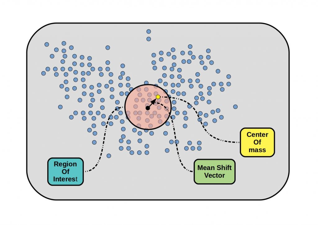
The first algorithm we want to introduce you to is Mean-Shift Clustering. With this you can find dense areas of data points according to the concept of kernel density estimation (KDE). The basis of the clustering is a circular sliding window, which moves towards higher density at each iteration. Within the window, the centers of each class are determined, called centroids.

The movement is now created by moving the center to the average of the points within the window. The density within the sliding window is thus proportional to the number of points within it. This motion continues until there is no direction in which the motion can take more points within the kernel.

Clustering Machine Learning Algorithms - Schematic and simplified representation of the Mean-Shift principle.
Clustering Machine Learning Algorithms – Mean-Shift Clustering Priciple

Hierarchical Cluster Analysis (HCA)

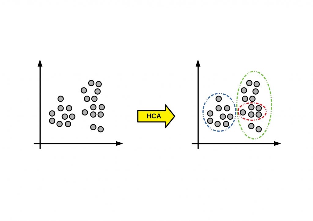
With HCA, clusters are formed based on empirical similarity measures of the data points. This means that the two most similar objects are assigned one after the other until all objects are in one cluster. This results in a tree-like structure. In contrast to the K-means algorithm, which we will discuss later, similarities between the clusters play a role. These are represented by a cluster distance. With K-means, only all objects within a collection are similar to each other, while they are dissimilar to objects in other clusters.

You can create an HCA in different ways. There are two elementary procedures, the top-down and the bottom-up. If you want to know more about Hierarchical Cluster Analysis, read this article.

Schematic and simplified representation of the HCA clustering  principle.
Clustering Machine Learning Algorithms – HCA Principle

Expectation-Maximization (EM) Clustering using Gaussian Mixture Models (GMM)

GMM basically assumes that the data points are Gaussian and not circular. The clusters are described by their mean and standard deviation. Each Gaussian distribution is randomly assigned to a single cluster and found using the Expectation-Maximization (EM) optimization algorithm. The probability of belonging to a cluster is then calculated for each data point. Thus, the closer a point is to the Gaussian center, the more likely it is then to belong to that cluster. Based on these probabilities, a new set of parameters for the Gaussian distributions is iteratively calculated. That is, the probabilities within a cluster are maximized.

K-Means clustering algorithms

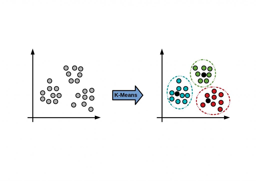
The k-Means algorithm described by MacQueen, 1967 goes back to the methods described by Lloyd, 1957 and Forgy, 1965. You can use the algorithm besides cluster analysis also for vector quantization. Here, a data set is partitioned into k groups with equal variance.

The number of clusters must be specified in advance. Each disjoint cluster is described by the average of all contained samples. The so-called cluster centroid.


Each centroid is updated to represent the average of its constituent instances. This is done until the assignment of instances to the clusters does not
changes any more. If you want to learn more about the K-means algorithm, check this out.

Schematic and simplified representation.of the kmeans clustering algorithm
K-Means Principle

Density-Based Spatial Clustering of Applications with Noise (DBSCAN)

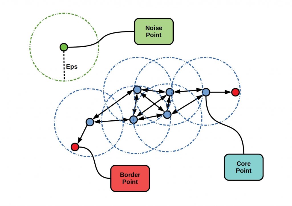
DBSCAN is a density-based cluster analysis with noise. From an arbitrary starting data point, neighborhood points are specified at a distance epsilon. Clustering then begins from a certain neighborhood data point count.

The current data point becomes the first point of the new cluster, or referred to as noise. In both cases, however, it is considered to be examined. The neighboring data points are then added to the cluster. Once all neighbors have been added, a new, unexamined point is called and processed. A new cluster is thus formed.

Schematic and simplified representation of the DBSCAN Clustering principle.
Clustering Machine Learning Algorithms – How DBSCAN works

The field of cluster algorithms is wide and everyone’s approach is different. You should be aware that there is no one solution. You have to consider each algorithm as another tool. Not every technique works equally well in every situation.

The key here is to always understand the basic approach of each algorithm you want to use. Build a small portfolio and get to know these techniques well. Once you master them, you should then add new ones. Knowing your own tools is crucial to avoid try and error and to gain control over your data. Remember: no result is a result. Your added value here is that even if an algorithm doesn’t work well on your data set, it will give you information about the data properties.

« Older posts